PHASE–TTC
From motion to time.
How long until contact? Two sensors measure motion. One causal system estimates the time.
RGB sees appearance. Event cameras record changes in brightness. PHASE–TTC combines their measurements to estimate signed time to contact.
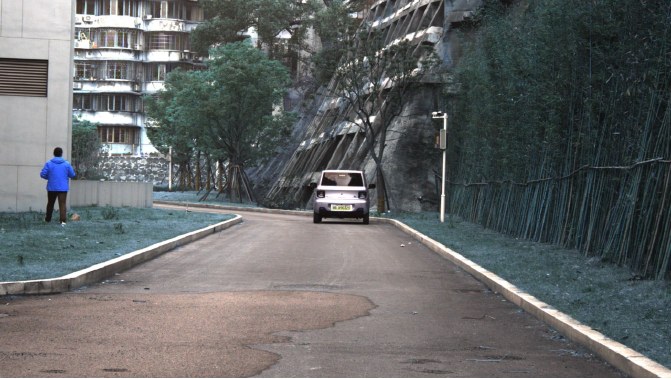
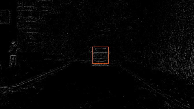
The same scene, through different measurements.
FCWD1:0007. Source and context in the paperA clock in the motion
An object growing in the image can reveal how quickly it is approaching.
Time-to-contact describes how soon contact would occur if relative motion continued. Scale change offers a useful cue under geometric assumptions, but rotation, occlusion and changing surfaces can break that connection.
The model works in phase space, a representation of relative scale change over a declared time interval, and converts its output back to seconds. Error in phase and error in seconds measure different things.
Follow a real scene
Two sensors, the same moment. Play the original RGB frames and recorded events, then inspect what each branch estimated.
EvTTC · CCRm, low speed · frozen TRAIN40 system · 6.1 seconds
The recording could not load. The still image and saved estimates remain available. Open the video
Both views share the recording clock. Their camera coordinates differ, so the views are shown side by side, without a spatial overlay.
The event view accumulates real brightness-change events over 100 ms. The colors show polarity; this is a rendering of sensor data, not a generated animation.
Recorded estimates
Query 1 / 16 t = 14.350 s
- Reference
- s
- RGB
- s
- Events
- s
- PHASE-TTC
- s
Jump to an evaluated instant
Values update only at the 16 saved queries. Between queries, the last recorded estimate remains visible. No predicted values are interpolated and no model runs in your browser.
- Reference
- RGB
- Events
- PHASE-TTC
Lines connect recorded samples to make the trend readable. Fusion can help or hurt at a particular instant; the full excerpt is shown.
Inspect every recorded value
| Elapsed | Reference | RGB | Events | PHASE-TTC |
|---|---|---|---|---|
| 0.00 s | 5.696 | 4.978 | 5.411 | 4.803 |
| 0.35 s | 5.287 | 5.074 | 4.693 | 4.576 |
| 0.70 s | 4.932 | 4.436 | 4.065 | 4.036 |
| 1.05 s | 4.595 | 4.604 | 4.366 | 4.254 |
| 1.40 s | 4.248 | 4.106 | 3.631 | 3.680 |
| 1.75 s | 3.958 | 3.529 | 3.561 | 3.289 |
| 2.10 s | 3.701 | 2.996 | 3.407 | 2.903 |
| 2.45 s | 3.452 | 2.995 | 2.768 | 2.732 |
| 2.80 s | 3.116 | 2.846 | 2.893 | 2.711 |
| 3.15 s | 2.845 | 2.523 | 2.580 | 2.312 |
| 3.85 s | 2.392 | 2.171 | 2.346 | 2.040 |
| 4.50 s | 2.033 | 1.921 | 2.320 | 1.876 |
| 4.85 s | 1.894 | 1.713 | 1.717 | 1.593 |
| 5.30 s | 1.756 | 1.848 | 2.228 | 1.905 |
| 5.70 s | 1.748 | 2.624 | 2.171 | 2.332 |
| 6.10 s | 2.112 | 2.461 | 5.016 | 2.600 |
These are saved outputs from the frozen TRAIN40 system in the 468-query transfer study, not the later adapted fusion. Object regions were supplied and the data had been exposed during development. The reference is the scenario TTC annotation. This excerpt is not a new benchmark or live-camera evaluation. Media and result provenance · EvTTC attribution and license.
Inside one prediction
Follow the data through every part of the architecture. The real inputs and saved outputs follow the query selected in the replay above.
A shared spatial frame
A shared spatial frame
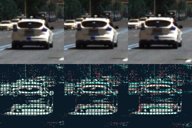
Each modality receives supplied object regions. A common crop keeps the same spatial scale across the observation endpoints, then resizes the samples to 128 × 128 pixels.
Real recorded input
Real RGB and event crops at the same observation endpoint. The animation visits the three endpoints; the sensors have separate coordinate systems. Crop colors preserve the model input channel order, which differs from the color-corrected camera replay. JPEG crops visualize the inputs; they are not lossless tensor files.
Supplied regions → common coordinates → image triplets
Why it is here
If every object were independently resized to fill its image, apparent growth could disappear. Preserving that growth keeps a useful motion cue.
From event times to twelve planes
From event times to twelve planes
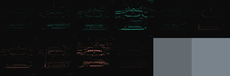
Each 100 ms window becomes five temporal bins for positive events and five for negative events. An event contributes to adjacent bins through linear interpolation. The region’s global log-count and log-rate add two spatially constant channels.
Real recorded input
Inspect all twelve planes
The actual encoded input at the selected query, rescaled per plane for display. Constant channels can look uniform. These are inputs, not learned activations.
(x, y, t, polarity) → 5 + 5 + 2 → 12 × 128 × 128
Why it is here
The network receives spatial measurements that retain polarity, timing and activity, rather than an unordered list of events.
The first motion estimate
The first motion estimate
R-A5 processes RGB pairs and E-A5 processes event representations. Each producer builds a learned pair token with 128 values and motion diagnostics, alongside a first TTC or phase estimate.
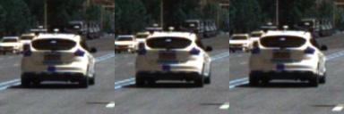
Real recorded input
The crops are real. The token and arrows are a structural diagram; intermediate activations were not saved for this replay.
Paired observations → R-A5 / E-A5 → token and motion estimate
Why it is here
This creates a separate measurement from each sensor before the system considers temporal history or cross-sensor correction.
Match at more than one scale
Match at more than one scale
R-C2F and E-C2F provide an additional motion estimate using local correspondences at coarse and fine feature resolutions. They run beside A5, not after it.
Coarse search
Fine search
Real crops illustrate the idea of scale. This diagram does not display the learned feature pyramid or measured correspondence vectors.
Local features → coarse and fine correspondence → a second estimate
Why it is here
A broad search can cover larger displacements; a finer search can refine local agreement. The two producers can disagree, and that disagreement becomes useful input to later stages.
A token needs a clock
A token needs a clock
PAIR-R and PAIR-E read each A5 token together with elapsed-time and observation-support fields. Their 133-value input produces an additional phase estimate for each sensor.
Symbolic fields show the computation, not saved values. A5, C2F and PAIR now provide three phase estimates per modality.
128 token values + 3 clock values + 2 support values → phase
Why it is here
The same visual change over a shorter interval implies different motion. Timing and valid support help the readout interpret the pair.
Refine each sensor through time
Refine each sensor through time
R-CTX and E-CTX use separate two-layer GRUs. Each reads 17 measurement features and four timing fields over up to eight valid observations. Their 160-value hidden states stay inside each branch.
The interactive trace uses saved RGB and event estimates from the selected query and earlier queries in the excerpt. Enable JavaScript to inspect those recorded samples.
This trace shows earlier saved context outputs in the excerpt, not the GRU hidden state or its exact internal slots.
Valid history at this query: RGB — / events —.
Measurements + their clocks → independent GRUs → refined RGB / event phase
Why it is here
History helps place a noisy or disagreeing measurement in context. Only available past observations can contribute; the 650 ms support span is not response latency.
Correct the RGB phase
Correct the RGB phase
The ninth component receives ten named fields from each branch. A compact 20 → 32 → 32 → 3 head predicts a correction anchored to RGB. It has 1,955 parameters; that is not the size of the full system.
From each sensor
The seconds above are saved final branch and fusion outputs. Intermediate raw phase fields and correction values are not recorded here.
10 RGB fields + 10 event fields → phase correction → refined phase
Why it is here
Fusion can use sensor disagreement, timing and history support without mixing opaque recurrent states. Its benefit must be measured: a correction can also make a prediction worse.
A signed estimate, with a reference
A signed estimate, with a reference
The corrected phase is mapped back to inverse TTC and then to seconds. Positive TTC represents approach; negative TTC represents recession. The output convention saturates near zero inverse TTC at ±60 s.
Absolute error in this query: 0.893 s
TTC = sign⁺(q) / max(|q|, 1/60)
Zero phase maps to +60 s by convention. Learned phase widths are not calibrated collision probabilities.
Phase → inverse TTC → signed seconds
Why it is here
Phase gives the system a motion representation; seconds make the result readable. Comparing with the recorded reference reveals the error for this query, not a general accuracy guarantee.
Nine fitted components: R-A5, E-A5, R-C2F, E-C2F, PAIR-R, PAIR-E, R-CTX, E-CTX and fusion. This explains their design roles; controlled ablations are needed to establish the contribution of each component. The displayed transfer queries were exposed during development.
Two paths. One estimate.
Nine fitted components turn independent motion estimates into a correction anchored in RGB.
Architecture and training in the paperMeasure motion
Each sensor has an A5 baseline producer and a coarse-to-fine C2F producer. Their shared spatial frame preserves apparent scale change. Object regions are supplied to the evaluated system.
Read the past
PAIR-R and PAIR-E extract phase features. Separate two-layer GRU refiners combine motion, timing and available history. Each prediction uses only observations available by its query time.
Fuse explicit quantities
The RGB-anchored head adjusts the RGB phase estimate using 20 named phase, timing and support features. It then converts phase into signed TTC. Learned hidden states stay within each modality.
1,955 trainable parameters in the correction head. This is not the size of the entire system.
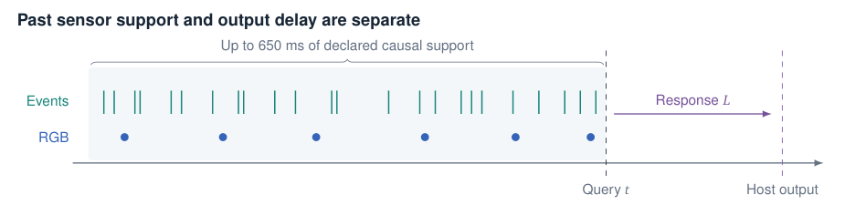
Inspect the full neural architecture
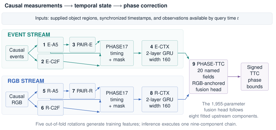
Inspect what reaches the fusion head
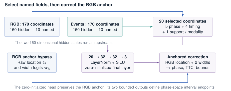
Learning with separated groups
Grouped out-of-fold predictions train the later stages. Five auxiliary rotations keep sequence groups separate during feature generation; deployment runs one chain. Earlier architecture-selection exposure and the shift from auxiliary training to the full refit remain limitations.
The benchmark result
20.49% lower Overall MiD than the published Garl-TTC reference.
Archived GarlTTC Test result, 28 October 2026. First among the three displayed submissions at that date.
Benchmark evidence in the paper| System | Score |
|---|---|
| PHASE–TTC | 35.80 |
| Garl-TTC | 45.03 |
6,762 scored tokens: 5,805 distinct physical queries and 957 aliases across twelve sequences. Both entries have 0% scorer-defined failures.
What this result establishes
MiD measures displacement in phase space, not error in seconds. A scorer failure is a nonfinite prediction or a predicted TTC magnitude below 0.1 s; zero failures does not mean zero missed collisions. The leaderboard does not standardize history, supplied localization, supervision or runtime. It does not isolate the contribution of events or any single component.
What changed this week
Quality-aware adaptation. Corrected local evaluation. Stronger controls.
The expanded edition adds experiments through 2 November. The original benchmark remains frozen.
Adaptation on EvTTC
Three small quality routers combine signed inverse-TTC estimates from neural and causal geometric experts. Each router has 688 trainable parameters; seeds 7, 13 and 21 form the delivered ensemble. The nine upstream models stay frozen.
Mean absolute error. Lower is better.
59.28% lower local MAE. Mean relative error decreases from 49.894242% to 17.249803%. The 365 road queries also improve, from 0.305401 to 0.185200 s MAE, so the aggregate change is not solely a Slider effect.
Local adaptation, with prior exposure
The routers fit 2,608 development queries. Although competition recordings are excluded from these optimizer updates, earlier experiments had already inspected them. Slider-750 still disagrees with the organizer’s evaluator. Both variants use the organizer-described interpolation of negative predictions for scoring only; archived signed predictions stay unchanged. These gains are not a new official score or independent generalization result.
Why the coverage statement changed
The earlier article reported output coverage for 434 queries without verified targets. Subsequent work corrected local target association and enabled a local accuracy comparison. This supersedes that coverage-only statement, while evaluator disagreement and development exposure still limit the interpretation.
The clock is part of the measurement
Actual observation cadence and the canonical phase interval are different quantities. Correcting that distinction gives a modest road change whose interval includes zero, and a larger change on one exposed Slider recording. Later router and refit controls fail their promotion gates. The cadence experiment does not replace the delivered adapter.
Canonical cadence intervention in the paperWhere fusion helps
Better tail error does not guarantee better average error.
A separate transfer study uses 468 development-exposed EvTTC queries with positive TTC. This is a different population from the 434-query adaptation above.
| Measure | RGB | PHASE–TTC |
|---|---|---|
| MAE | 1.015 | 1.023 |
| p95 | 3.799 | 3.243 |
| Errors > 10 s | 2 | 5 |
All 95% intervals for paired differences in mean, median and p95 absolute error include zero. This does not establish a universal event-camera benefit. Learned phase widths also require empirical calibration before being interpreted as probabilities.
Transfer analysis in the paperWhat did not work
Negative results shaped the system. The original JEPA hypothesis is part of the research history, not a claim about the final estimator.
Prediction needs a control
A fixed-teacher pilot compared static distillation, one-step prediction and shuffled futures across three seeds. Neither prespecified superiority test passed under the sequence-bootstrap criterion. Log-height-change error is dimensionless, not TTC error in seconds. These experiments do not establish a JEPA benefit.
Correct physics is not enough
Physical descriptors, normal-flow measurements and three-frame surfaces were tested against matched system baselines. Several interpretable routes worsened complete-system TTC. Correct equations and better intermediate measurements do not by themselves establish a better final estimate.
Detection is a separate task
The eAP detection study raises aligned development mAP from 0.05702 to 0.06204 by reranking fixed proposals. Its official AP is 0.05130, without a paired baseline test submission. An eight-frame detector–tracker–TTC replay demonstrates the interface, not independent end-to-end TTC accuracy.
Time to an answer
A causal estimate still has to arrive on time.
Response target
Measured p95
The five-second, 50 Hz replay completed 250 single-object updates with numerical parity and no drops. But 201 responses met or exceeded 20 ms. Latency starts at scheduled arrival and ends with all required TTC outputs on the host.
RTX 5070 Ti Laptop GPU, preloaded RAW data, disk I/O excluded. This is not a live-camera or sustained multi-object result. Other runtime measurements remain separate because their workloads and measurement boundaries differ.
Follow the evidence
The expanded 65-page edition brings the method, executed results, rejected candidates and reproducibility record together.
Expanded edition: 2 November 2026
The standalone LaTeX needs the figures included in the complete source ZIP.